ML Mathematical Theory

Deep learning fundamentals — regularization, optimization, normalization, attention math, and activation functions

Core Architecture & Signal Flow

Activation Functions · Transformer Attention Math · Weight Initialization

Activation Functions

Activation functions introduce nonlinearity into the network. Without them, stacking linear layers would collapse to a single linear transformation — no matter how deep the network, it could only learn linear relationships.

Activation	Formula	Output Range	Zero-Centered?	Compute Cost	Vanishing Gradient	Sparsity	Primary Use
Sigmoid	1 / (1 + e⁻ˣ)	(0, 1)	No	High (exp)	High risk	No	Binary classification output
Tanh	(eˣ − e⁻ˣ) / (eˣ + e⁻ˣ)	(−1, 1)	Yes	High (exp)	Moderate	No	RNN hidden layers
ReLU	max(0, x)	[0, ∞)	No	Low (threshold)	Low (x>0)	Yes (zeros negatives)	Default hidden layers

Weight Initialization Strategies

Why not initialize all weights to 0?

Symmetry problem: every neuron computes the same output and receives the same gradient — the network never differentiates. The derivative of the loss w.r.t. each weight is αx, where α is the same constant for all weights, so they all update identically and the hidden layer collapses to a single neuron.

Xavier / Glorot (for Sigmoid / Tanh)

Sample weights from a distribution with:

var(w) = 1/n_in or 2 / (n_in + n_out)

n_in = fan-in, n_out = fan-out. Keeps var(output) = var(input) across layers. Works because sigmoid/tanh are nearly linear near 0.

He / Kaiming (for ReLU)

Sample weights from a distribution with:

var(w) = 2 / n_in

n_in = fan-in. The factor of 2 compensates for ReLU zeroing ~50% of activations, which would otherwise halve signal variance every layer.

Transformer Attention Math

Scaled dot-product attention, Q/K/V projections, multi-head splitting, masking, and the √d_k variance derivation are covered in depth in the Transformers Cheatsheet.

Learning Dynamics & Convergence

Loss Functions · Optimization + Momentum · Vanishing + Exploding Gradients

Loss Functions

Entropy H(P)

Complexity of the true distribution P. If labels are fixed, this is constant — minimizing cross-entropy is the same as minimizing KL.

KL Divergence D_KL(P‖Q)

Extra information lost when using predicted distribution Q to approximate true distribution P. A measure of distance between distributions. Not symmetric.

Cross-Entropy H(P, Q)

Total cost of using Q to represent P. H(P, Q) = H(P) + D_KL(P‖Q).

Standard Classification → Cross-Entropy

True labels P are constant — minimizing CE is equivalent to minimizing KL. Simpler and sufficient.

RL / Knowledge Distillation → KL Divergence

Target distribution is also moving (soft labels, policy updates) — KL directly measures how Q tracks the shifting P.

Vanishing & Exploding Gradients

Why do deep networks suffer — and how do residual connections fix it?

During backprop, the gradient at layer k is a product of many Jacobians. If activation derivatives (e.g. sigmoid) are <1, the product shrinks exponentially → vanishing gradient.

ResNet Solution: y = f(x) + x

Gradient becomes f′(x) + 1 — the +1 provides a constant highway for gradients.
Faster convergence: direct path for both gradients and information.
Smoother landscape: enables training of very deep networks.

Optimization & Momentum

Optimization algorithms update model weights to minimize the loss. Momentum accumulates a velocity vector — incorporating a weighted history of past gradients to move faster through flat regions and resist oscillation in narrow valleys.

SGD (Stochastic Gradient Descent)

Computes gradient on random mini-batches. Stochasticity helps escape local minima and pushes weights toward flat minima (better generalization). Simple but slow and sensitive to learning rate.

Adam (Adaptive Moment Estimation)

1st moment m: Exponential moving average of gradients — direction and velocity.
2nd moment v: Moving average of squared gradients — intensity. Large gradient → shrink LR. Small gradient → accelerate LR.
Adaptive per-parameter LR. Faster convergence, but can generalize worse than SGD.

Optimizer	Speed	LR Tuning	Memory	Generalization
SGD	Slow	Hard	None	Excellent
SGD + Momentum	Faster	Medium	Velocity	Good
Adam	Fastest	Easy	Velocity + Intensity	Can overfit

Regularization & Generalization

Bias-Variance Trade-off · L1 Lasso vs L2 Ridge · Dropout

Regularization (L1 & L2)

What is regularization?

Adds a penalty term to the loss to discourage overly large weights:

L_total = L_data(ŷ, y) + λ · Ω(w)

λ controls regularization strength; Ω(w) is the weight penalty.

Why does it prevent overfitting?

Sensitivity: Smaller weights → less sensitive slopes → noise causes smaller output changes.
Geometrically: Restricts search space — forces the model to capture only the strongest signals.
Hessian: Adds a bowl to the loss landscape, shifting minima toward smoother, more generalizable regions.

L1 vs L2

L1 — Lasso

Ω(w) = Σ|wᵢ|

Constant gradient (±1) near zero — pushes weights all the way to exactly 0. Produces sparse models.

L2 — Ridge

Ω(w) = Σwᵢ²

Gradient scales with weight (2w) — damps near zero but rarely reaches exactly 0. Produces small, smooth weights.

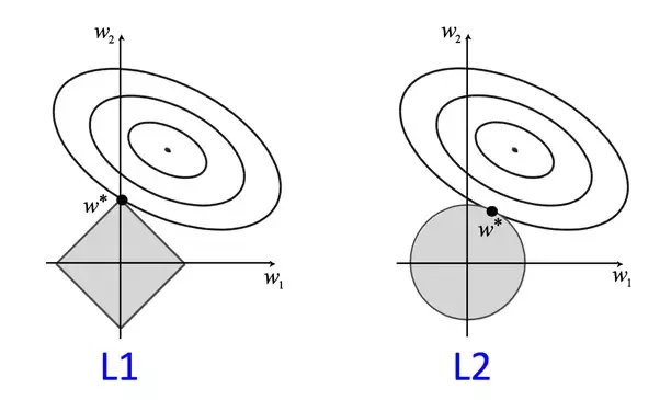
Geometric comparison of L1 (diamond) and L2 (circle) constraint regions.

L1's diamond corners lie on the axes — w* lands where a weight = 0. L2's circle intersects the contour off-axis, shrinking but not zeroing.

Bias-Variance Tradeoff

Bias is error from overly simplistic assumptions. Variance is error from excessive sensitivity to training data. Increasing model complexity tends to decrease bias but increase variance. The goal is the sweet spot that minimizes total error on unseen data.

Overfitting — High Variance

Too complex. Memorizes noise. Low bias, high variance — good on train, poor on test.

Underfitting — High Bias

Too simple. Misses the pattern. High bias, low variance — poor on both train and test.

2x2 target diagrams: low/high bias vs low/high variance.

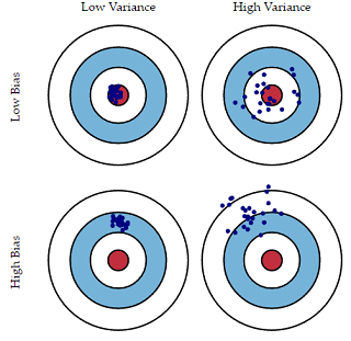
Low bias = predictions near center. Low variance = predictions tightly clustered. Ideal: top-left (low bias, low variance).

Dropout

Prevents co-adaptation of neurons and reduces overfitting. Srivastava et al., 2014

Dropout is a regularization technique that randomly zeros out individual neurons during each training step using a Bernoulli mask. This prevents neurons from co-adapting — relying too heavily on specific neighbors — and forces the network to learn more distributed, redundant representations that generalize better to unseen data. At inference, dropout is turned off and activations are rescaled to match expected training values.

Bernoulli Mask

Each neuron is independently kept with probability (1−p) and zeroed with probability p. A fresh mask is sampled every forward pass during training, so no two passes see the same sub-network.

Inverted Dropout Scaling

Without scaling, turning off dropout at inference would double the expected activation magnitude. To fix this, activations are divided by (1−p) during training — keeping the expected value of each neuron's output equal to its value at inference, where all neurons are active.

Python

class MyDropout(nn.Module):
    def __init__(self, p=0.5):
        super().__init__()
        self.p = p

    def forward(self, x):
        if not self.training or self.p == 0:
            return x
        # Bernoulli mask: 1 = keep, 0 = drop
        mask = (torch.rand_like(x) > self.p).float()
        # Inverted scaling keeps expected value = x
        return x * mask / (1 - self.p)

Monte Carlo Dropout (Bayesian Interpretation)

By keeping dropout on at inference and running many forward passes with different masks, the spread of outputs approximates a probability distribution over predictions. The mean is the model's best guess; the variance measures epistemic uncertainty — how confident the model is based on what it has seen during training. Useful in safety-critical settings where knowing "I'm not sure" matters.

Transformer-specific variants

DropPath: Drops entire residual branches rather than individual neurons — acts as a stronger structural regularizer for deep networks.
Attention Dropout: Applied directly to the softmax attention weight matrix, preventing the model from always attending to the same set of tokens.
Variational Dropout: Reuses the same mask across all time steps in a sequence, preserving positional structure while still regularizing.

Normalization & Stability

Batch Normalization — mean/variance shift, γ and β affine transforms

Batch Normalization

Normalizes activations per mini-batch; stabilizes and accelerates training. Ioffe & Szegedy, 2015

Batch Normalization standardizes each layer's activations to have zero mean and unit variance across the mini-batch, then applies learned affine parameters γ (scale) and β (shift) to restore expressiveness. This decouples each layer from the scale of its inputs, allowing higher learning rates, faster convergence, and reduced sensitivity to weight initialization.

x̂ = (x − μ_B) / √(σ²_B + ε) → y = γ·x̂ + β

μ_B and σ²_B are the batch mean and variance. ε is a small constant for numerical stability. γ and β are learned parameters that let the model undo the normalization if needed.

Internal Covariate Shift

As weights update during training, the distribution of inputs to each layer shifts — layers deeper in the network must constantly re-adapt to a moving target. BN normalizes each layer's output so downstream layers receive stable, consistent distributions, enabling higher learning rates and faster, more reliable convergence.

Smoother Loss Landscape

A more recent explanation: BN makes the loss function Lipschitz-stable, meaning the gradient doesn't change drastically from one step to the next. This allows the optimizer to take larger, more confident steps without overshooting, improving both stability and speed.

Running Stats at Inference

During training, BN uses the current mini-batch's mean and variance. At inference, batch sizes may be small or 1 — making batch statistics unreliable. Instead, BN tracks a running mean and running variance via exponential moving average during training and uses those fixed values at inference.

μ_run ← momentum · μ_run + (1 − momentum) · μ_batch

Smaller momentum = slower updates (more stable); larger = faster but noisier.

Why BN + Dropout interact badly

Dropout randomly zeros neurons during training, which shifts the mean and variance of the activations that BN then observes. The running statistics BN accumulates are computed on these half-zeroed distributions. At inference, dropout is off and all neurons are active — so the true activation distribution is different from what BN learned, causing a train/inference mismatch that degrades performance.

Batch Normalization — Code

Python

def batch_norm_forward(x, gamma, beta, eps=1e-5, momentum=0.9,
                        running_mean=None, running_var=None, training=True):
    N, D = x.shape
    if running_mean is None: running_mean = np.zeros(D)
    if running_var  is None: running_var  = np.ones(D)

    if training:
        batch_mean = np.mean(x, axis=0)
        batch_var  = np.var(x,  axis=0)
        x_hat = (x - batch_mean) / np.sqrt(batch_var + eps)
        out   = gamma * x_hat + beta
        # Exponential moving average
        running_mean = momentum * running_mean + (1 - momentum) * batch_mean
        running_var  = momentum * running_var  + (1 - momentum) * batch_var
        cache = (x, x_hat, batch_mean, batch_var, gamma, eps)
        return out, cache, running_mean, running_var
    else:
        x_hat = (x - running_mean) / np.sqrt(running_var + eps)
        return gamma * x_hat + beta